
Welcome to Luciano Iess's Homepage
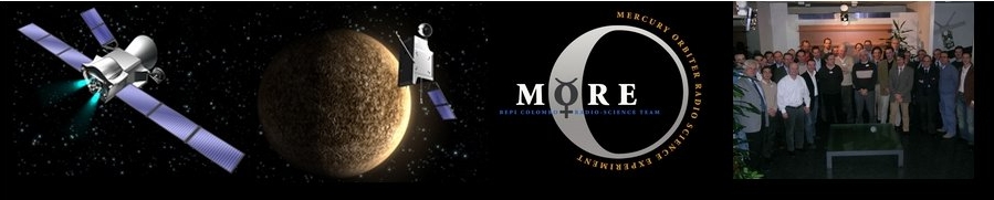
On the left: the BepiColombo spacecraft, the MORE - Mercury Orbiter Radioscience Experiment - logo and team. BepiColombo is an ESA mission devoted to the scientific exploration of Mercury. Launch: 20 October 2018.
Messages
Abbreviations:
- SMS = Space Missions and Systems
- AS = Space Environment
IMPORTANT ANNOUNCEMENT:
The course on Space Missions and Systems will start on Tuesday 27 Feb.
Results of the 2022 Orbit Determination Challenge
Giulia Nejat 2 pt
Andrea Vittori 2 pt
Mariano Conti 1 pt
Paolo Pagnozzi 1 pt
Roberto Santori 1 pt
Congratulations to the winners and all participants, whether you succeeded or not!
Challenge 2021
Winners
First place: Pasquale Tartaglia
Second place: Chiara Pazzelli, Ariele Zurria
Third place: Chiara Pozzi, Giuliano Vinci, Alessandro Beolchi
The Challenge is a valid replacement for HW1 for the students in green in this list.
Congratulations to all participants! We received many very good answers. I hope everyone learned something on OD and enjoyed solving the problem.
Luciano Iess
Homework 1
Results of HW1
Color codes:
Green = pass
Red = fail
Yellow = pass, but with some errors. It is strongly advised to do the challenge, answering the first questions (1-2, TBD). The second hpmework must be a "full green".
Problem
Observable data file
Deadline: Sunday 11 April 23:59:59. The text and the observable file is also available on Google Classroom. Use Classroom to upload your solution (a pdf file) and working code. If you are not on Classroom, use email (to me and paolo.cappuccio@uniroma1.it). Be concise and go right to the point. A well done set of figures is worth a thousand words.
Information regarding the SMS and AS courses:
We will use the Zoom platform, on my NEW personal virtual room.
To access it, use the following invitation and link:
Luciano Iess is inviting you to a scheduled Zoom meeting:
Topic: Luciano Iess's Personal Meeting Room
Join Zoom Meeting:
https://uniroma1.zoom.us/j/8534489651?pwd=WEcxRWlGS0JUaG5Mb253L0NveHdvZz09
Meeting ID: 853 448 9651
Passcode: 250498
You must enter the room with your FIRST NAME and LAST NAME. You will not be admitted to the virtual classroom with nicknames.
**** Space Missions and Systems
Matlab codes for the coherent demodulator: version 1 (shown in class) and version 2
Challenge 2020 - Results
1st place: not awarded
2nd place: Fabiani, Gubernari
3rd place: Pallarés Chamorro, Di Muzio (+1 pt.)
The challenge is a valid replacement for HW1 for the following students:
Capocchiano, Di Francesca, Di Muzio, Maioli, Mattei, Mereu, Moretti, Paci, Silvestri, Sponsillo
Congratulations to all participants! Many of you did quite a good job.
Follow the link on the left panel to get the instructions for the remote exam sessions.
For detailed instructions you may also download this pdf document (last update 25/5).
Please visit this website for updates.
This is all experimental. If you have suggestions on better ways to continue the course, do not hesitate to contact me.
Luciano Iess
STAGE AND THESIS - NEW OPPORTUNITIES (updated 8 May 2020) - See link on the left
-------------------
Space Missions and Systems class 12 March 2020
Using the Matlab code and the concepts you learned during the course, answer the following questions:
1) Which observables are most sensitive to x_0?
2) Which observables are most sensitive to v_0?
3) How does the state accuracy (standatd deviation) vary with h? Make a plot or a table.
4) Try to change one of the model parameters (k_1,k_2,m). Does the filter converge? Why?
5) Implement the MVE in the Spring-Mass Matlab script.
6) How do the standard deviations of the estimated state variables change?
7) Try to simulate your own observed observables (you can find the code in the file “spring_main_batch.m”
8) Using only one type of observables at a time, what is the maximum level of noise that guarrantees convergence?
The spring-mass Matlab code has been uploaded in the folder "Class Notes"/"Space Missions and Systems"/"Supplementary Material".
The previous version is also available in the same folder. There the observable quantities are generated in the matlab code. You can play with the noise level.
----------------------
NEW: Work and stage opportunities - see link on the left. (21/5/2019).
::::::::::::::::::::::::::::::::::::::::::::::::::::::::::::::::::::::::::::::::::::::::::::::::::::
*** Plumbing the depth of Jupiter's winds
Here is the link to the recent paper on Nature and some of its echoes in the news:
Iess et al. "Measurement of Jupiter's asymmetric gravity field", Nature, 555, 220-222 (2018)
International coverage
Scientific American (really good)
The Hindustan Times (India)
Coverage in Italy
----------------------------------------------------------------
*** Short course on Matlab: Download the full zip file here
Luciano Iess: "The Attraction of Gravity" - Jean Dominique Cassini Medal Lecture at the European Geosciences Union - Vienna, April 25, 2017. Video recording
*** New supporting material:
Matlab codes for batch and sequential estimation (spring-mass system) in Class Notes - Supporting Material
*** An interesting link: Cassini behind the scenes
**** Space Missions and Systems
Matlab code for the coherent demodulator
___________________________________________________________
For updated information you may follow me on Twitter (luciano_iess)
*** Seminars at Beijing Institute of Tracking and Telecommunications Technology (BITTT):
Seminar 1: Deep Space Navigation Systems: Where Do We Stand?
Seminar 2: The European Delta-DOR Correlator
Seminar 3: BepiColombo, the ESA Mission To Mercury; MORE: Geodesy, Geophysics, Navigation
Seminar 4 and 5: The Scientific Use of Deep Space Tracking Systems; Radio Science in Deep Space Missions
***Tour of Robledo's DNS facilities. The visit to the Robledo and Cebreros tracking complexes was an interesting and profitable experience for all of us. Follow the link to see some photos.
__________
Frequently Asked Question (FAQ)
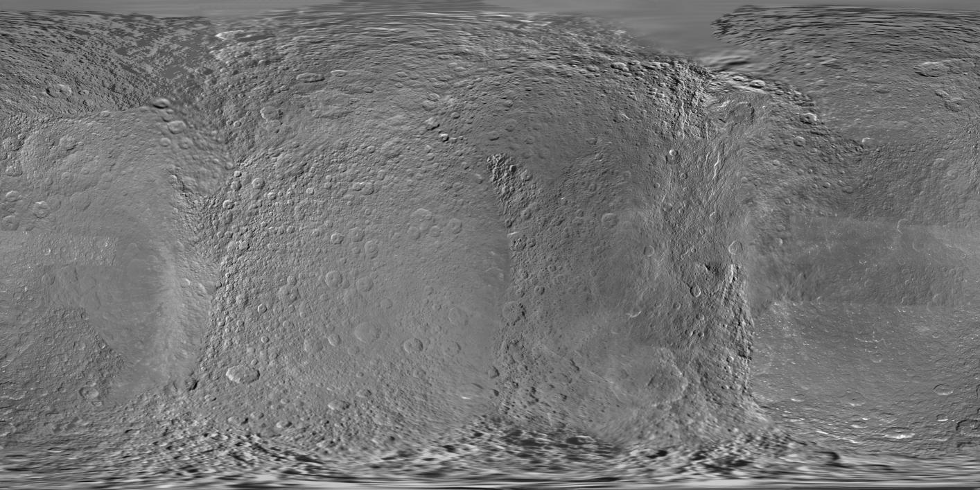
Map of Rhea